Membuat Program Regresi Logistik Dengan Python Menggunakan Anaconda(Spyder)

Pada hari jumat yang lalu, saya telah membagikan sebuah tutorial untuk membuat program regresi logistik dengan python menggunakan anaconda.

Nah, pada kesempatan kali ini saya akan kembali membagikan source code untuk membuat program regresi logistik. 

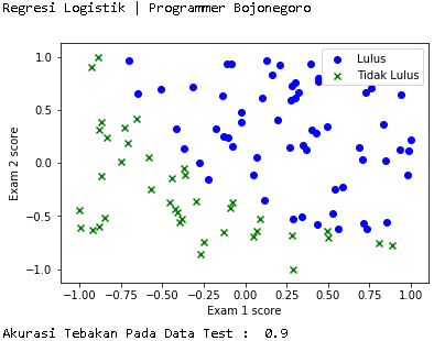
Namun berbeda dengan tutorial kemarin, kali ini output yang dihasilkan berbentuk grafik seperti berikut.

Berikut source code program regresi logistik dengan python menggunakan anacoda.

# -*- coding: utf-8 -*-
"""
This program performs two different logistic regression implementations on two
different datasets of the format [float,float,boolean], one
implementation is in this file and one from the sklearn library. The program
then compares the two implementations for how well the can predict the given outcome
for each input tuple in the datasets.

Program ini melakukan dua regresi logistik yang berbeda implementasi pada dua
dataset yang berbeda dari format [float, float, boolean], salah satu
implementasi ini dalam file ini dan satu dari library sklearn. Program
kemudian membandingkan dua penerapan untuk seberapa baik dapat memprediksi hasil yang diberikan
untuk setiap input tupel dalam dataset.

Created on Fri Dec 22 01:20:02 2017

@author: Tubianto
*Website: Programmer Bojonegoro | programmerbojonegoro.blogspot.co.id
"""

import math
import numpy as np
import pandas as pd
from pandas import DataFrame
from sklearn import preprocessing
from sklearn.linear_model import LogisticRegression
from sklearn.cross_validation import train_test_split
from numpy import loadtxt, where
from pylab import scatter, show, legend, xlabel, ylabel
# scale larger positive and values to between -1,1 depending on the largest
# value in the data

# skala besar positif dan nilai-nilai antara - 1,1 tergantung pada terbesar
# nilai data
min_max_scaler = preprocessing.MinMaxScaler(feature_range=(-1,1))
df = pd.read_csv("data.csv", header=0)

# clean up data

# membersihkan data
df.columns = ["grade1","grade2","label"]

#x = df["label"].map(lambda x: float(x.rstrip(';')))

# formats the input data into two arrays, one of independant variables
# and one of the dependant variable

# format input data ke dalam array dua, salah satu variabel yang independen
# dan salah satu variabel tergantung
X = df[["grade1","grade2"]]
X = np.array(X)
X = min_max_scaler.fit_transform(X)
Y = df["label"].map(lambda x: float(x.rstrip(';')))
Y = np.array(Y)

# if want to create a new clean dataset 
##X = pd.DataFrame.from_records(X,columns=['grade1','grade2'])
##X.insert(2,'label',Y)
##X.to_csv('data2.csv')

# Jika ingin membuat dataset bersih baru
##X = pd. DataFrame.from_records(X,columns=['grade1','grade2'])
##X.insert(2,'label',Y)
##X.to_csv('data2.csv')

# creating testing and training set

# membuat pengujian dan pelatihan set
X_train,X_test,Y_train,Y_test = train_test_split(X,Y,test_size=0.1)

# visualize data, uncomment "show()" to run it

# memvisualisasikan data, tanda komentar "show()" untuk menjalankan
print ('Regresi Logistik | Programmer Bojonegoro')
pos = where(Y == 1)
neg = where(Y == 0)
scatter(X[pos, 0], X[pos, 1], marker='o', c='b')
scatter(X[neg, 0], X[neg, 1], marker='x', c='g')
xlabel('Exam 1 score')
ylabel('Exam 2 score')
legend(['Lulus', 'Tidak Lulus'])
show()

##The sigmoid function adjusts the cost function hypotheses to adjust the algorithm proportionally for worse estimations

##The sigmoid fungsi menyesuaikan hipotesis fungsi biaya untuk menyesuaikan algoritma proporsional untuk lebih buruk estimasi
def Sigmoid(z):
 G_of_Z = float(1.0 / float((1.0 + math.exp(-1.0*z))))
 return G_of_Z 

##The hypothesis is the linear combination of all the known factors x[i] and their current estimated coefficients theta[i] 
##This hypothesis will be used to calculate each instance of the Cost Function

##The Hipotesis adalah kombinasi linear semua faktor yang diketahui x [i] dan mereka saat ini diperkirakan koefisien theta [i]
##This Hipotesis akan digunakan untuk menghitung setiap contoh fungsi biaya
def Hypothesis(theta, x):
 z = 0
 for i in xrange(len(theta)):
  z += x[i]*theta[i]
 return Sigmoid(z)

##For each member of the dataset, the result (Y) determines which variation of the cost function is used
##The Y = 0 cost function punishes high probability estimations, and the Y = 1 it punishes low scores
##The "punishment" makes the change in the gradient of ThetaCurrent - Average(CostFunction(Dataset)) greater

##For setiap anggota dataset, hasil (Y) menentukan variasi fungsi biaya digunakan
##The Y = 0 biaya fungsi menghukum estimasi probabilitas tinggi, dan Y = 1 it menghukum nilai rendah
##The "hukuman" membuat perubahan dalam gradien ThetaCurrent - Average(CostFunction(Dataset)) yang lebih besar
def Cost_Function(X,Y,theta,m):
 sumOfErrors = 0
 for i in xrange(m):
  xi = X[i]
  hi = Hypothesis(theta,xi)
  if Y[i] == 1:
   error = Y[i] * math.log(hi)
  elif Y[i] == 0:
   error = (1-Y[i]) * math.log(1-hi)
  sumOfErrors += error
 const = -1/m
 J = const * sumOfErrors
 print ('cost is ', J)
 return J

##This function creates the gradient component for each Theta value 
##The gradient is the partial derivative by Theta of the current value of theta minus 
##a "learning speed factor aplha" times the average of all the cost functions for that theta
##For each Theta there is a cost function calculated for each member of the dataset

##This fungsi menciptakan komponen gradien untuk setiap nilai Theta
##The gradien adalah turunan parsial oleh Theta dari nilai saat ini dari theta minus
##a "belajar kecepatan faktor aplha" kali rata-rata semua fungsi biaya untuk theta itu
##For Theta setiap ada adalah fungsi biaya dihitung untuk masing-masing anggota dataset
def Cost_Function_Derivative(X,Y,theta,j,m,alpha):
 sumErrors = 0
 for i in xrange(m):
  xi = X[i]
  xij = xi[j]
  hi = Hypothesis(theta,X[i])
  error = (hi - Y[i])*xij
  sumErrors += error
 m = len(Y)
 constant = float(alpha)/float(m)
 J = constant * sumErrors
 return J

##For each theta, the partial differential 
##The gradient, or vector from the current point in Theta-space (each theta value is its own dimension) to the more accurate point, 
##is the vector with each dimensional component being the partial differential for each theta value

##For theta setiap, diferensial parsial
##The gradien, atau vektor dari titik saat ini di Theta-ruang (setiap nilai theta adalah dimensi sendiri) ke titik lebih akurat,
##is vektor dengan komponen masing-masing dimensi yang diferensial parsial untuk setiap nilai theta
def Gradient_Descent(X,Y,theta,m,alpha):
 new_theta = []
 constant = alpha/m
 for j in xrange(len(theta)):
  CFDerivative = Cost_Function_Derivative(X,Y,theta,j,m,alpha)
  new_theta_value = theta[j] - CFDerivative
  new_theta.append(new_theta_value)
 return new_theta

##The high level function for the LR algorithm which, for a number of steps (num_iters) finds gradients which take 
##the Theta values (coefficients of known factors) from an estimation closer (new_theta) to their "optimum estimation" which is the
##set of values best representing the system in a linear combination model

##The fungsi tingkat tinggi untuk algoritma LR yang, untuk sejumlah langkah-langkah (num_iters) menemukan gradien yang mengambil
##the theta nilai (koefisien faktor yang diketahui) dari perkiraan lebih dekat (new_theta) untuk mereka "estimasi optimal" yang
##set nilai-nilai terbaik mewakili sistem dalam model kombinasi linear
def Logistic_Regression(X,Y,alpha,theta,num_iters):
 m = len(Y)
 for x in xrange(num_iters):
  new_theta = Gradient_Descent(X,Y,theta,m,alpha)
  theta = new_theta
  if x % 100 == 0:
   #here the cost function is used to present the final hypothesis of the model in the same form for each gradient-step iteration
            
          #here fungsi biaya digunakan untuk menyajikan hipotesis akhir model dalam bentuk yang sama untuk setiap perulangan gradien-langkah
   Cost_Function(X,Y,theta,m)
   print ('theta ', theta) 
   print ('cost is ', Cost_Function(X,Y,theta,m))
 Declare_Winner(theta)

##This method compares the accuracy of the model generated by the scikit library with the model generated by this implementation

##This metode membandingkan ketepatan model yang dihasilkan oleh Perpustakaan scikit dengan model yang dihasilkan oleh pelaksanaan ini
'''
def Declare_Winner(theta):
 score = 0
 winner = ""
 #first scikit LR is tested for each independent var in the dataset and its prediction is compared against the dependent var
 #if the prediction is the same as the dataset measured value it counts as a point for thie scikit version of LR
 scikit_score = clf.score(X_test,Y_test)
 length = len(X_test)
 for i in xrange(length):
   prediction = round(Hypothesis(X_test[i],theta))
  answer = Y_test[i]
  if prediction == answer:
   score += 1
 #the same process is repeated for the implementation from this module and the scores compared to find the higher match-rate
 my_score = float(score) / float(length)
 if my_score > scikit_score:
  print ('You won!')
 elif my_score == scikit_score:
  #print 'Its a tie!'
 else:
  #print 'Scikit won.. :('
 print ('Your score: ', my_score)
 print ('Scikits score: ', scikit_score) 
'''
# These are the initial guesses for theta as well as the learning rate of the algorithm
# A learning rate too low will not close in on the most accurate values within a reasonable number of iterations
# An alpha too high might overshoot the accurate values or cause irratic guesses
# Each iteration increases model accuracy but with diminishing returns,
# and takes a signficicant coefficient times O(n)*|Theta|, n = dataset length

# Ini adalah perkiraan awal untuk theta serta tingkat belajar algoritma
# Tingkat belajar yang terlalu rendah tidak akan menutup pada nilai-nilai yang paling akurat dalam jumlah yang wajar dari iterasi
# Alfa terlalu tinggi mungkin overshoot nilai akurat atau menyebabkan irratic menebak
# Setiap iterasi meningkatkan akurasi model tetapi dengan kembali yg berkurang,
# dan mengambil signficicant koefisien kali O(n) * | Theta |, n = panjang dataset
#initial_theta = [0,0]
#alpha = 0.1
#iterations = 1000
##Logistic_Regression(X,Y,alpha,initial_theta,iterations)

##Logistic_Regression(X,Y,alpha,initial_theta,iterations)

# train scikit learn model

# Kereta scikit belajar model
clf = LogisticRegression()
clf.fit(X_train,Y_train)
print ('Akurasi Tebakan Pada Data Test : ', clf.score(X_test,Y_test))

Alhamdulillah, itulah source code untuk membuat program regresi logistik dengan python menggunakan anaconda(spyder).

Semoga bermanfaat dan menambah wawasan temen-temen semua.

Share this post